Analyzing functions: lab 3
© 2005 Ben Bolker
This lab will be somewhat shorter in terms of " R stuff"
than the previous labs, because more of the new material
is algebra and calculus than R commands.
Try to do a reasonable amount of the work with paper
and pencil before resorting to messing around in R.
derivatives
ifelse for thresholds
1 Numerical experimentation: plotting curves
Here are the R commands used to generate Figure 1. They
just use curve(), with add=FALSE (the default,
which draws a new plot) and add=TRUE (adds the curve
to an existing plot), particular
values of from and to, and various graphical parameters
(ylim, ylab, lty).
> curve(2 * exp(-x/2), from = 0, to = 7, ylim = c(0, 2), ylab = "")
> curve(2 * exp(-x), add = TRUE, lty = 4)
> curve(x * exp(-x/2), add = TRUE, lty = 2)
> curve(2 * x * exp(-x/2), add = TRUE, lty = 3)
> text(0.4, 1.9, expression(paste("exponential: ", 2 * e^(-x/2))),
+     adj = 0)
> text(4, 0.7, expression(paste("Ricker: ", x * e^(-x/2))))
> text(4, 0.25, expression(paste("Ricker: ", 2 * x * e^(-x/2))),
+     adj = 0)
> text(2.8, 0, expression(paste("exponential: ", 2 * e^(-x))))
The only new thing in this figure is the
use of expression() to add a mathematical
formula to an R graphic. text(x,y,"x^2")
puts x^2 on the graph at position (x,y);
text(x,y,expression(x^2)) (no quotation marks)
puts x2 on the graph. See ?plotmath or
?demo(plotmath) for (much) more information.
An alternate way of plotting the exponential parts of this
curve:
> xvec = seq(0, 7, length = 100)
> exp1_vec = 2 * exp(-xvec/2)
> exp2_vec = 2 * exp(-xvec)
> plot(xvec, exp1_vec, type = "l", ylim = c(0, 2), ylab = "")
> lines(xvec, exp2_vec, lty = 4)
or, since both exponential vectors are the
same length, we could cbind() them
together and use matplot():
> matplot(xvec, cbind(exp1_vec, exp2_vec), type = "l", ylab = "")
Finally, if you needed to use sapply()
you could say:
> expfun = function(x, a = 1, b = 1) {
+     a * exp(-b * x)
+ }
> exp1_vec = sapply(xvec, expfun, a = 2, b = 1/2)
> exp2_vec = sapply(xvec, expfun, a = 2, b = 1)
The advantage of curve() is that you
don't have to define any vectors: the advantage
of doing things the other way arises when
you want to keep the vectors around to do
other calculations with them.
Exercise 1*: Construct a curve
that has a maximum at (x=5, y=1). Write the
equation, draw the curve in R, and explain
how you got there.
1.1 A quick digression: ifelse() for piecewise functions
The ifelse() command in R is useful for constructing
piecewise functions. Its basic syntax is
ifelse(condition,value_if_true,value_if_false),
where condition is a logical vector
(e.g. x>0), value_if_true is a vector
of alternatives to use if condition is
TRUE, and value_if_false is a vector
of alternatives to use if condition is
FALSE. If you specify just one value, it
will be expanded (recycled in R jargon)
to be the right length.
A simple example:
> x = c(-25, -16, -9, -4, -1, 0, 1, 4, 9, 16, 25)
> ifelse(x < 0, 0, sqrt(x))
[1] 0 0 0 0 0 0 1 2 3 4 5
These commands produce a warning message, but it's OK
to ignore it since you know you've taken care of the
problem (if you said sqrt(ifelse(x<0,0,x)) instead
you wouldn't get a warning: why not?)
Here are some examples of using ifelse() to generate
(1) a simple threshold; (2) a Holling type I or
"hockey stick"; (3) a more complicated piecewise model
that grows exponentially and then decreases linearly;
(4) a double-threshold model.
> op = par(mfrow = c(2, 2), mgp = c(2, 1, 0), mar = c(4.2, 3, 1,
+     1))
> curve(ifelse(x < 2, 1, 3), from = 0, to = 5)
> curve(ifelse(x < 2, 2 * x, 4), from = 0, to = 5)
> curve(ifelse(x < 2, exp(x), exp(2) - 3 * (x - 2)), from = 0,
+     to = 5)
> curve(ifelse(x < 2, 1, ifelse(x < 4, 3, 5)), from = 0, to = 5)
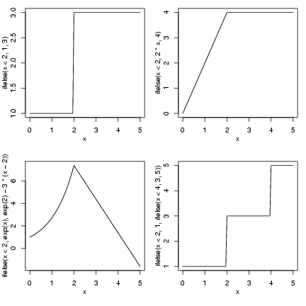 The double-threshold example (nested
ifelse() commands) probably needs
more explanation. In words, this command would
go "if x is less than 2, set y to 1; otherwise
(x ł 2), if x is less than 4 (i.e. 2 Ł x < 4), set y to 3;
otherwise (x ł 4), set y to 5".
The double-threshold example (nested
ifelse() commands) probably needs
more explanation. In words, this command would
go "if x is less than 2, set y to 1; otherwise
(x ł 2), if x is less than 4 (i.e. 2 Ł x < 4), set y to 3;
otherwise (x ł 4), set y to 5".
2 Evaluating derivatives in R
R can evaluate derivatives, but it is not
very good at simplifying them.
In order for R to know that you really
mean (e.g) x^2 to be a mathematical
expression and not a calculation for R to
try to do (and either fill in the current
value of x or give an error is
x is undefined), you have to specify
it as expression(x^2); you
also have to tell R (in quotation marks)
what variable you want to differentiate
with respect to:
> d1 = D(expression(x^2), "x")
> d1
2 * x
Use eval() to fill in
a list of particular
values for which you want a numeric answer:
> eval(d1, list(x = 2))
[1] 4
Taking the second derivative:
> D(d1, "x")
[1] 2
(As of version 2.0.1,) R knows how
to take the derivatives of expressions including
all the basic arithmetic operators;
exponentials and logarithms; trigonometric
inverse trig, and hyperbolic trig functions;
square roots; and normal (Gaussian)
density and cumulative density functions;
and gamma and log-gamma functions.
You're on your own for anything else
(consider using a symbolic algebra package
like Mathematica or Maple, at least to check
your answers, if your problem is very complicated).
deriv() is a slightly more complicated
version of D() that is useful for incorporating
the results of differentiation into functions:
see the help page.
3 Figuring out the logistic curve
The last part of this exercise is an example of figuring out a
function - Chapter 3 did this for the exponential,
Ricker, and Michaelis-Menten functions
The population-dynamics form of the logistic
equation is
|
n(t) = |
K
|
1+ |
ć
č
|
K
n(0)
|
-1 |
ö
ř
|
exp(-r t) |
|
|
| (1) |
where K is carrying
capacity, r is intrinsic population growth rate, and n(0) is
initial density.
At t=0, e-rt=1 and this reduces to n(0)
(as it had better!)
Finding the derivative with respect to time is pretty ugly,
but it will to reduce to something you may already know.
Writing the equation as
n(t) = K ·(stuff)-1
and using the chain rule we get
n˘(t) = K ·(stuff)-2 ·d(stuff)/dt
(stuff=1+(K/n(0)-1)exp(-rt)).
The derivative d(stuff)/dt
is (K/n(0)-1) ·-r exp(-rt).
At t=0, stuff=K/n(0),
and d(stuff)/dt=-r(K/n(0)-1).
So this all comes out to
|
K ·(K/n(0))-2 ·-r (K/(n0)-1) = -r n(0)2/K ·(K/(n0)-1) = r n(0) (1-n(0)/K) |
|
which should be reminiscent of intro. ecology:
we have rediscovered, by working backwards
from the time-dependent solution, that the
logistic equation arises from a linearly
decreasing per capita growth rate.
If n(0) is small we can do better than
just getting the intercept and slope.
Exercise 2*: show that
if n(0) is very small (and t is not too big),
n(t) » n(0) exp(r t). (Start by showing that
K/n(0) e-rt dominates all
the other terms in the denominator.)
If t is small, this reduces (because
ert » 1+rt) to
n(t) » n(0) + r n(0) t,
a linear increase with slope rn(0).
Convince yourself that this matches
the expression we got for the derivative
when n(0) is small.
For large t, convince yourself tha
the value of the
function approaches K and
(by revisiting
the expressions for the derivative above)
that the slope approaches zero.
The half-maximum occurs when the
denominator (also known as stuff above) is
2; we can solve stuff=2 for t
(getting to (K/n(0)-1) exp(-rt) = 1
and taking logarithms on both sides)
to get t=log(K/n(0)-1)/r.
We have (roughly) three options:
- Use curve():
> r = 1
> K = 1
> n0 = 0.1
> curve(K/(1 + (K/n0 - 1) * exp(-r * x)), from = 0, to = 10)
(note that we have to use x and
not t in the expression for the logistic).
- Construct the time vector by hand
and compute a vector of population values
using vectorized operations:
> t_vec = seq(0, 10, length = 100)
> logist_vec = K/(1 + (K/n0 - 1) * exp(-r * t_vec))
> plot(t_vec, logist_vec, type = "l")
- write our own function for the logistic
and use sapply():
> logistfun = function(t, r = 1, n0 = 0.1, K = 1) {
+     K/(1 + (K/n0 - 1) * exp(-r * t))
+ }
> logist_vec = sapply(t_vec, logistfun)
When we use this
function, it will no longer matter how
r, n0 and K are
defined in the workspace: the
values that R uses in logistfun()
are those that we define in the
call to the function.
> r = 17
> logistfun(1, r = 2)
[1] 0.4508531
> r = 0
> logistfun(1, r = 2)
[1] 0.4508531
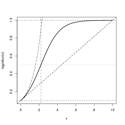
We can do more with this plot: let's see if our
conjectures are right.
Using abline()
and curve() to add horizontal lines to a plot
to test our estimates of starting value and ending value,
vertical and horizontal lines that intersect at the half-maximum,
a line with the intercept and initial linear slope, and
a curve corresponding to the initial exponential increase:
> curve(logistfun(x), from = 0, to = 10, lwd = 2)
> abline(h = n0, lty = 2)
> abline(h = K, lty = 2)
> abline(h = K/2, lty = 3)
> abline(v = -log(n0/(K - n0))/r, lty = 4)
> r = 1
> abline(a = n0, b = r * n0 * (1 - n0/K), lty = 5)
> curve(n0 * exp(r * x), from = 0, lty = 6, add = TRUE)
 Exercise 3*:
Plot and analyze the function G(N)=[RN/((1+aN)b)],
(the Shepherd function), which is
a generalization of the Michaelis-Menten function.
What are the effects of the R and a parameters
on the curve?
For what parameter
values does this function become equivalent to
the Michaelis-Menten function?
What is the behavior (value, initial slope) at N=0?
What is the behavior (asymptote [if any], slope) for large N,
for b=0, 0 < b < 1, b=1, b > 1?
Define an R function for the Shepherd function (call it
shep). Draw a plot or plots
showing the behavior for the ranges above, including lines that
show the initial slope.
Extra credit: when does the function have a maximum between 0 and
Ą? What is the height of the
maximum when it occurs?
(Hint: when you're figuring out whether a fraction is zero
or not, you don't have to think about the denominator at all.)
The calculus isn't that hard, but you may also use the
D() function in R.
Draw horizontal and vertical lines onto the graph to test your
answer.
Exercise 4*:
Reparameterize the Holling type III functional response
(f(x)=ax2/(1+bx2)) in terms of its asymptote and half-maximum.
Exercise 5*:
Figure out the correspondence between the
population-dynamic parameterization of the
logistic function (eq. 1:
parameters r, n(0), K)
and the statistical parameterization
(f(x)=exp(a+bx)/(1+exp(a+bx)):
parameters a, b).
Convince yourself you got the right answer
by plotting the logistic with a=-5, b=2
(with lines), figuring out the equivalent
values of K, r, and n(0), and then plotting the
curve with both equations to make sure it overlaps.
Plot the statistical version with lines
(plot(...,type="l") or curve(...)
and then add the population-dynamic version with
points (points() or curve(...,type="p",add=TRUE)).
Small hint: the population-dynamic version
has an extra parameter, so one of r, n(0), and
K will be set to a constant when you translate
to the statistical version.
Big hint: Multiply the
numerator and denominator of the statistical form
by exp(-a) and the numerator and denominator
of the population-dynamic form by exp(rt),
then compare the forms of the equations.
Exercise 3*:
Plot and analyze the function G(N)=[RN/((1+aN)b)],
(the Shepherd function), which is
a generalization of the Michaelis-Menten function.
What are the effects of the R and a parameters
on the curve?
For what parameter
values does this function become equivalent to
the Michaelis-Menten function?
What is the behavior (value, initial slope) at N=0?
What is the behavior (asymptote [if any], slope) for large N,
for b=0, 0 < b < 1, b=1, b > 1?
Define an R function for the Shepherd function (call it
shep). Draw a plot or plots
showing the behavior for the ranges above, including lines that
show the initial slope.
Extra credit: when does the function have a maximum between 0 and
Ą? What is the height of the
maximum when it occurs?
(Hint: when you're figuring out whether a fraction is zero
or not, you don't have to think about the denominator at all.)
The calculus isn't that hard, but you may also use the
D() function in R.
Draw horizontal and vertical lines onto the graph to test your
answer.
Exercise 4*:
Reparameterize the Holling type III functional response
(f(x)=ax2/(1+bx2)) in terms of its asymptote and half-maximum.
Exercise 5*:
Figure out the correspondence between the
population-dynamic parameterization of the
logistic function (eq. 1:
parameters r, n(0), K)
and the statistical parameterization
(f(x)=exp(a+bx)/(1+exp(a+bx)):
parameters a, b).
Convince yourself you got the right answer
by plotting the logistic with a=-5, b=2
(with lines), figuring out the equivalent
values of K, r, and n(0), and then plotting the
curve with both equations to make sure it overlaps.
Plot the statistical version with lines
(plot(...,type="l") or curve(...)
and then add the population-dynamic version with
points (points() or curve(...,type="p",add=TRUE)).
Small hint: the population-dynamic version
has an extra parameter, so one of r, n(0), and
K will be set to a constant when you translate
to the statistical version.
Big hint: Multiply the
numerator and denominator of the statistical form
by exp(-a) and the numerator and denominator
of the population-dynamic form by exp(rt),
then compare the forms of the equations.
File translated from
TEX
by
TTH,
version 3.67.
On 14 Sep 2005, 16:42.