| Licensed under the Creative Commons attribution-noncommercial license ( http://creativecommons.org/licenses/by-nc/3.0/). Please share & remix noncommercially, mentioning its origin. |
These notes are based in part on course materials by former TAs Colleen Webb, Jonathan Rowell and Daniel Fink at Cornell, Professors Lou Gross (University of Tennessee) and Paul Fackler (NC State University), and on the book Getting Started with Matlab by Rudra Pratap (Oxford University Press). They also draw on the documentation supplied with R. They parallel, but go into more depth than, the chapter supplement for the book Ecological Models and Data in R.
You can find many other similar introductions scattered around the web, or in the “contributed documentation” section on the R web site ( http://cran.r-project.org/other-docs.html). This particular version is limited (it has similar coverage to Sections 1 and 2 of the Introduction to R that comes with R) and targets biologists who are neither programmers nor statisticians.
R is an object-oriented scripting language that combines
R is an open source project, available for free download via the Web. Originally a research project in statistical computing (Ihaka and Gentleman, 1996), it is now managed by a development team that includes a number of well-regarded statisticians, and is widely used by statistical researchers (and a growing number of theoretical ecologists and ecological modelers) as a platform for making new methods available to users. The commercial implementation of S (called S-PLUS) offers an Office-style “point and click” interface that R lacks. For our purposes, however, the advantage of this front-end is outweighed by the fact that R is built on a faster and much less memory-hungry implementation of S and is easier to interface with other languages (and is free!). A standard installation of R also includes extensive documentation, including an introductory manual (≈ 100 pages) and a comprehensive reference manual (over 1000 pages). (There is a graphical front-end for parts of R, called “R commander” (Rcmdr for short), available at the R site, but we will not be using it in this class.)
If R is already installed on your computer, you can skip this section.
The main source for R is the CRAN home page http://cran.r-project.org. You can get the source code, but most users will prefer a precompiled version. To get one of these from CRAN:
R should work well on any reasonably modern computer. Version 2.5.1 requires MacOS X 10.4.4 (or higher) or Windows 95 (or higher), or just about any version of Linux; it can also be compiled on other versions of Unix. Windows XP or higher is recommended. R moves quickly: if possible, you should make sure you have upgraded to the most recent version available, or at least that your version isn’t more than about a year old.
The standard distributions of R include several packages, user-contributed suites of add-on functions (unfortunately, the command to load a package into R is library!). These Notes use some packages that are not part of the standard distribution. In general, you can install additional packages from within R using the Packages menu, or the install.packages command. (See below.)
For Windows or MacOS, install R by launching the downloaded file and following the on-screen instructions. At the end you’ll have an R icon on your desktop that you can use to launch the program. Installing versions for Linux or Unix is slightly more complicated, which will not bother the corresponding users. For doing anything more than very simple examples, we recommend the Tinn-R ( http://www.sci-views.org/Tinn-R) or Notepad++ ( notepad-plus.sourceforge.net/) editors as better Windows interfaces than the built-in console: in particular, these editors have syntax highlighting, which colors R commands and allows you to identify missing parentheses, quotation marks, etc..
 If you are using R on a machine where you have sufficient permissions,
you may want to edit some of your graphical user interface (GUI) options.
If you are using R on a machine where you have sufficient permissions,
you may want to edit some of your graphical user interface (GUI) options.
 Just click on the icon on your desktop, or in the Start menu (if you
allowed the Setup program to make either or both of these). If you lose
these shortcuts for some reason, you can search for the executable file
Rgui.exe on your hard drive, which will probably be somewhere like
Program Files\R\R-x.y.z\bin\Rgui.exe. If you are using Tinn-R, first start
Tinn-R, then go to …
Just click on the icon on your desktop, or in the Start menu (if you
allowed the Setup program to make either or both of these). If you lose
these shortcuts for some reason, you can search for the executable file
Rgui.exe on your hard drive, which will probably be somewhere like
Program Files\R\R-x.y.z\bin\Rgui.exe. If you are using Tinn-R, first start
Tinn-R, then go to …
You can stop R from the File menu ( ), or you can stop it by typing q() at
the command prompt (if you type q by itself, you will get some confusing output
which is actually R trying to tell you the definition of the q function; more on
this later).
), or you can stop it by typing q() at
the command prompt (if you type q by itself, you will get some confusing output
which is actually R trying to tell you the definition of the q function; more on
this later).
When you quit, R will ask you if you want to save the workspace (that is, all of the variables you have defined in this session); for now (and in general), say “no” in order to avoid clutter.
Should an R command seem to be stuck or take longer than you’re willing to wait, click on the stop sign on the menu bar or hit the Escape key (in Unix, type Control-C).
 When you start R it opens the console window. The console has a few basic
menus at the top; check them out on your own. The console is also where you
enter commands for R to execute interactively, meaning that the command is
executed and the result is displayed as soon as you hit the Enter key. For
example, at the command prompt >, type in 2+2 and hit Enter; you will
see
When you start R it opens the console window. The console has a few basic
menus at the top; check them out on your own. The console is also where you
enter commands for R to execute interactively, meaning that the command is
executed and the result is displayed as soon as you hit the Enter key. For
example, at the command prompt >, type in 2+2 and hit Enter; you will
see
(When cutting and pasting from this document to R, don’t include the text for the command prompt (>).)
To do anything complicated, you have to store the results from calculations by assigning them to variables, using = or <-. For example:
R automatically creates the variable a and stores the result (4) in it, but it doesn’t print anything. This may seem strange, but you’ll often be creating and manipulating huge sets of data that would fill many screens, so the default is to skip printing the results. To ask R to print the value, just type the variable name by itself at the command prompt:
(the [1] at the beginning of the line is just R printing an index of element numbers; if you print a result that displays on multiple lines, R will put an index at the beginning of each line. print(a) also works to print the value of a variable.) By default, a variable created this way is a vector, and it is numeric because we gave R a number rather than some other type of data (e.g. a character string like "pxqr"). In this case a is a numeric vector of length 1, which acts just like a number.
You could also type a=2+2; a, using a semicolon to put two or more commands on a single line. Conversely, you can break lines anywhere that R can tell you haven’t finished your command and R will give you a “continuation” prompt (+) to let you know that it doesn’t think you’re finished yet: try typing
to see what happens (you will sometimes see the continuation prompt when you don’t expect it, e.g. if you forget to close parentheses). If you get stuck continuing a command you don’t want—e.g. you opened the wrong parentheses—just hit the Escape key or the stop icon in the menu bar to get out.
Variable names in R must begin with a letter, followed by letters or numbers. You can break up long names with a period, as in very.long.variable.number.3, or an underscore (_), but you can’t use blank spaces in variable names (or at least it’s not worth the trouble). Variable names in R are case sensitive, so Abc and abc are different variables. Make variable names long enough to remember, short enough to type. N.per.ha or pop.density are better than x and y (too short) or available.nitrogen.per.hectare (too long). Avoid c, l, q, t, C, D, F, I, and T, which are either built-in R functions or hard to tell apart.
R does calculations with variables as if they were numbers. It uses +, -, *, /, and ^ for addition, subtraction, multiplication, division and exponentiation, respectively. For example:
Even though R did not display the values of x and y, it “remembers” that it assigned values to them. Type x; y to display the values.
You can retrieve and edit previous commands. The up-arrow ( ↑ ) key (or Control-P) recalls previous commands to the prompt. For example, you can bring back the second-to-last command and edit it to
(experiment with the other arrow keys (↓, →, ←), Home and End keys too). This will save you many hours in the long run.
You can combine several operations in one calculation:
Parentheses specify the order of operations. The command
is not the same as the one above; rather, it is equivalent to C=A + 2*(sqrt(A)/A) + 5*sqrt(A).
The default order of operations is: (1) parentheses; (2) exponentiation, or powers, (3) multiplication and division, (4) addition and subtraction (“pretty please excuse my dear Aunt Sally”).
| b = 12-4/2^3 | gives | 12 - 4/8 = 12 - 0.5 = 11.5 |
| b = (12-4)/2^3 | gives | 8/8 = 1 |
| b = -1^2 | gives | -(1^2) = -1 |
| b = (-1)^2 | gives | 1 |
In complicated expressions you might start off by using parentheses to specify explicitly what you want, such as b = 12 - (4/(2^3)) or at least b = 12 - 4/(2^3) ; a few extra sets of parentheses never hurt anything, although when you get confused it’s better to think through the order of operations rather than flailing around adding parentheses at random.
R also has many built-in mathematical functions that operate on variables (Table 1 shows a few).
|
Exercise 2.1 : Using editing shortcuts wherever you can, have R compute the values of
 and compare it with (1 -
 )-1 (If any square brackets [] show
up in your web browser’s rendition of these equations, replace them
with regular parentheses ().)
)-1 (If any square brackets [] show
up in your web browser’s rendition of these equations, replace them
with regular parentheses ().)
 e-x2∕2
, for values of x = 1 and
x = 2 (R knows π as pi.) (You can check your answers against the
built-in function for the normal distribution; dnorm(1) and dnorm(2)
should give you the values for the standard normal for x = 1 and
x = 2.)
e-x2∕2
, for values of x = 1 and
x = 2 (R knows π as pi.) (You can check your answers against the
built-in function for the normal distribution; dnorm(1) and dnorm(2)
should give you the values for the standard normal for x = 1 and
x = 2.)R has a help system, although it is generally better for providing detail or reminding you how to do things than for basic “how do I …?” questions.
(where foo is the name of the function you are interested in) in the console window (e.g., try ?sin).
By default, R’s help system only provides information about functions that are in the base system and packages that you have loaded with library (see below).
Try out one or more of these aspects of the help system.
Other (on-line) help resources Paul Johnson’s “R tips” web page ( http://pj.freefaculty.org/R/Rtips.html) answers a number of “how do I …?” questions, although it’s out of date in some places. The R “wiki” ( http://wiki.r-project.org) is a newer venue for help information. The R tips page is (slowly) being moved over to the wiki, which will eventually (we hope) contain a lot more information. You can also edit the wiki and add your own pages!
Also see:
Exercise 3.1 : Do an Apropos on sin via the Help menu, to see what it does. Now enter the command
and see what that does (answer: help.search pulls up all help pages that include ‘sin’ anywhere in their title or text. Apropos just looks at the name of the function).
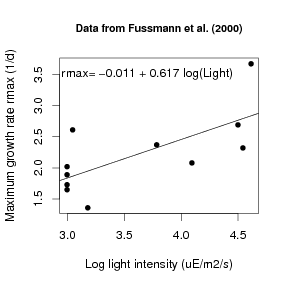
To get a feel for working in R we’ll fit a straight-line model (linear regression) to data. Below are some data on the maximum growth rate rmax of laboratory populations of the green alga Chlorella vulgaris as a function of light intensity (μE per m2 per second). These experiments were run during the system-design phase of the study reported by Fussmann et al. (2000).
Light: 20, 20, 20, 20, 21, 24, 44, 60, 90, 94, 101
rmax: 1.73, 1.65, 2.02, 1.89, 2.61, 1.36, 2.37, 2.08, 2.69, 2.32, 3.67
To analyze these data in R, first enter them as numerical vectors:
The function c combines the individual numbers into a vector. Try recalling (with ↑) and modifying the above command to
and see the error message you get: in order to create a vector of specified numbers, you must use the c function. Don’t be afraid of error messages: the answer to “what would happen if I …?” is usually “try it and see!”
To see a histogram of the growth rates enter hist(rmax), which opens a graphics window and displays the histogram. There are many other built-in statistics functions: for example mean(rmax) computes you the mean, and sd(rmax) and var(rmax) compute the standard deviation and variance, respectively. Play around with these functions, and any others you can think of.
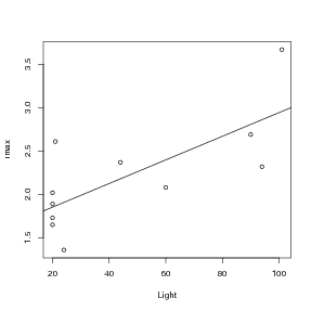
To see how light intensity affects algal rate of increase, type
to plot rmax (y) against Light (x). A linear regression would seem like a reasonable model for these data. Don’t close this plot window: we’ll soon be adding to it.
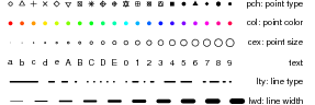
R’s default plotting character is an open circle. Open symbols are generally better than closed symbols for plotting because it is easier to see where they overlap, but you could include pch=16 in the plot command if you wanted closed circles instead. Figure 1 shows several more ways to adjust the appearance of lines and points in R.
To perform linear regression we create a linear model using the lm (linear model) function:
(Note that the variables are in the opposite order from the plot command, which is plot(x,y), whereas the linear model is read as “model rmax as a function of light”.)
The lm command produces no output at all, but it creates fit as an object, i.e. a data structure consisting of multiple parts, holding the results of a regression analysis with rmax being modeled as a function of Light. Unlike most statistics packages, R rarely produces automatic summary output from an analysis. Statistical analyses in R are done by creating a model, and then giving additional commands to extract desired information about the model or display results graphically.
To get a summary of the results, enter the command summary(fit). R sets up model objects (more on this later) so that the function summary “knows” that fit was created by lm, and produces an appropriate summary of results for an lm object:
[If you’ve had (and remember) a statistics course the output will make sense to you. The table of coefficients gives the estimated regression line as rmax = 1.58 + 0.0136 × Light, and associated with each coefficient is the standard error of the estimate, the t-statistic value for testing whether the coefficient is nonzero, and the p-value corresponding to the t-statistic. Below the table, the adjusted R-squared gives the estimated fraction of the variance explained by the regression line, and the p-value in the last line is an overall test for significance of the model against the null hypothesis that the response variable is independent of the predictors.]
You can add the regression line to the plot of the data with a function taking fit as its input (if you closed the plot of the data, you will need to create it again in order to add the regression line):
(abline, pronounced “a b line”, is a general-purpose function for adding lines to a plot: you can specify horizontal or vertical lines, a slope and an intercept, or a regression model: ?abline).
You can get the coefficients by using the coef function:
You can also “interrogate” fit directly. Type names(fit) to get a list of the components of fit, and then use the $ symbol to extract components according to their names.
For more information (perhaps more than you want) about fit, use str(fit) (for structure). You can get the regression coefficients this way:
It’s good to be able to look inside R objects when necessary, but all other things being equal you should prefer (e.g.) coef(x) to x$coefficients.
While R works perfectly well out of the box, there are interfaces that can make your R experience easier. Editors such as Tinn-R (Windows: http://www.sciviews.org/Tinn-R/), Kate (Linux: http://kate-editor.org), or Emacs/ESS (cross-platform: http://ess.r-project.org/ will color R commands and quoted material, allow you to submit lines or blocks of R code to an R session, and give hints about function arguments: the standard MacOS interface has all of these features built in. Graphical interfaces such as JGR (cross-platform: http://rosuda.org/JGR/) or SciViews (Windows: http://www.sciviews.org/SciViews-R/) include similar editors and have extra functions such as a workspace browser for looking at all the variables you have defined. (All of these interfaces, which are designed to facilitate R programming, are in a different category from Rcmdr, which tries to simplify basic statistics in R.) If you are using Windows or Linux I would strongly recommend that, once you have tried R a little bit, you download at least an R-aware editor and possibly a GUI to make your life easier. Links to all of these systems, and more, can be found at http://www.r-project.org/GUI/.
Modeling and complicated data analysis are often much easier if you use scripts, which are a series of commands stored in a text file. The Windows and MacOS versions of R both have basic script editors: you can also use Windows Notepad or Wordpad, or a more featureful editor like PFE, Xemacs, or Tinn-R: you should not use MS Word.
Most programs for working with models or analyzing data follow a simple pattern of program parts:
For example, a script file might
Even for relatively simple tasks, script files are useful for building up a calculation step-by-step, making sure that each part works before adding on to it.
Tips for working with data and script files (sounding slightly scary but just trying to help you avoid common pitfalls):
Changing your working directory is more efficient in the long run, if you save all the script and data files for a particular project in the same directory and switch to that directory when you start work.
If you have a shortcut defined for R on your desktop (or in the Start menu) you can permanently change your default working directory by right-clicking on the shortcut icon, selecting Properties, and changing the starting directory to somewhere like (for example) My Documents/R work.
As a first example, the file Intro1.R has the commands from the interactive regression analysis. Important: before working with an example file, create a personal copy in some location on your own computer. We will refer to this location as your temp folder. At the end of a lab session you must move files onto your personal disk (or email them to yourself).
Now open your copy of Intro1.R. In your editor, select and Copy the entire text of the file, and then Paste the text into the R console window (Ctrl-C and Ctrl-V as shortcuts). This has the same effect as entering the commands by hand into the console: they will be executed and so a graph is displayed with the results. Cut-and-Paste allows you to execute script files one piece at a time (which is useful for finding and fixing errors). The source function allows you to run an entire script file, e.g.
You can also source files by pointing and clicking via the File menu on the console window.
Another important time-saver is loading data from a text file. Grab copies of Intro2.R and ChlorellaGrowth.txt from the web page to see how this is done. In ChlorellaGrowth.txt the two variables are entered as columns of a data matrix. Then instead of typing these in by hand, the command
reads the file (from the current directory) and puts the data values into the variable X; header=TRUE specifies that the file includes column names. Note that as specified above you need to make sure that R is looking for the data file in the right place …either move the data file to your current working directory, or change the line so that it points to the actual location of the data file.
Extract the variables from X with the commands
Think of these as shorthand for “Light = everything in column 1 of X”, and “rmax = everything in column 2 of X” (we’ll learn about working with data matrices later). From there on out it’s the same as before, with some additions that set the axis labels and add a title.
Exercise 5.1 Make a copy of Intro2.R under a new name, and modify the copy so that it does linear regression of algal growth rate on the natural log of light intensity, LogLight=log(Light), and plots the data appropriately. You should end up with a graph that resembles Figure 3. (Hint: when you switch from light intensity to log light intensity, the range on your x axis will change and you will have to change the x position at which you plot the growth rate equation.)
|
|
Exercise 5.2 Run Intro2.R, then enter the command plot(fit) in the console and follow the directions in the console. Figure out what just happened by entering ?plot.lm to bring up the Help page for the function plot.lm that carries out a plot command for an object produced by lm. (This is one example of how R uses the fact that statistical analyses are stored as model objects. fit “knows” what kind of object it is (in this case an object of type lm), and so plot(fit) invokes a function that produces plots suitable for an lm object.) Answer: R produced a series of diagnostic plots exploring whether or not the fitted linear model is a suitable fit to the data. In each of the plots, the 3 most extreme points (the most likely candidates for “outliers”) have been identified according to their sequence in the data set.
Exercise 5.3 The axes in plots are scaled automatically, but the outcome is not always ideal (e.g. if you want several graphs with exactly the same axis limits). You can use the xlim and ylim arguments in plot to control the limits:
will draw the graph with the x-axis running from x1 to x2, and using ylim=c(y1,y2) within the plot command will do the same for the y-axis.
Create a plot of growth rate versus light intensity with the x-axis running from 0 to 120 and the y-axis running from 1 to 4.
Exercise 5.4 You can place several graphs within a single figure by using the par function (short for “parameter”) to adjust the layout of the plot. For example, the command
divides the plotting area into 2 rows and 3 columns. As R draws a series of graphs, it places them along the top row from left to right, then along the next row, and so on. mfcol=c(2,3) has the same effect except that R draws successive graphs down the first column, then down the second column, and so on.
Save Intro2.R with a new name and modify the program as follows. Use mfcol=c(2,1) to create graphs of growth rate as a function of Light, and of log(growth rate) as a function of log(Light) in the same figure. Do the same again, using mfcol=c(1,2).
Exercise 5.5 * Use ?par to read about other plot control parameters that you use par to set (you should definitely skim — this is one of the longest help files in the whole R system!). Then draw a 2 × 2 set of plots, each showing the line y = 5x + 3 with x running from 3 to 8, but with 4 different line styles and 4 different line colors.
Exercise 5.6 * Modify one of your scripts so that at the very end it saves the plot to disk. In Windows you can do this with savePlot, otherwise with dev.print. Use ?savePlot, ?dev.print to read about these functions. Note that the argument filename can include the path to a folder; for example, in Windows you can use filename="c:/temp/Intro2Figure".
(These are really exercises in using the help system, with the bonus that you learn some things about plot. (Let’s see, we know plot can graph data points (rmax versus Light and all that). Maybe it can also draw a line to connect the points, or just draw the line and leave out the points. That would be useful. So let’s try ?plot and see if it says anything about lines …Hey, it also says that graphical parameters can be given as arguments to plot, so maybe I can set line colors inside the plot command instead of using par all the time …) The help system can be quite helpful (amazingly enough) once you get used to it and get in the habit of using it often.)
The main point is not to be afraid of experimenting; if you have saved your previous commands in a script file, there’s almost nothing you can break by trying out commands and inspecting the results.
R has many extra packages that provide extra functions. You may be able to install new packages from a menu within R. You can always type
(for example — this installs the plotrix package). You can install more than one package at a time:
(c stands for “combine”, and is the command for combining multiple things into a single object.) If the machine on which you use R is not connected to the Internet, you can download the packages to some other medium (such as a flash drive or CD) and install them later, using Install from local zip file in the menu or
If you do not have permission to install packages in R’s central directory, R will may ask whether you want to install the packages in a user-specific directory. Go ahead and say yes.
You will frequently get a warning message something like Warning message: In file.create(f.tg) : cannot create file ’.../packages.html’, reason ’Permission denied’. Don’t worry about this; it means the package has been installed successfully, but the main help system index files couldn’t be updated because of file permissions problems.
If you install the emdbook package first (install.packages("emdbook")), load the package (library(emdbook)), and then run the command get.emdbook.packages() (you do need the empty parentheses) it will install these packages for you automatically.
(R2WinBUGS is an exception to R’s normally seamless cross-platform operation: it depends on a Windows program called WinBUGS. WinBUGS will also run on Linux or MacOS [on Intel hardware], with the help of a program called WINE (we’ll deal with this later).)
It will save time if you install these packages now.
Some of the important functions and packages (collections of functions) for statistical modeling and data analysis are summarized in Table 2. Venables and Ripley (2002) give a good practical (although somewhat advanced) overview, and you can find a list of available packages and their contents at CRAN, the main R website ( http://www.cran.r-project.org — select a mirror site near you and click on Package sources). For the most part, we will not be concerned here with this side of R.
|
Vectors and matrices (1- and 2-dimensional rectangular arrays of numbers) are pre-defined data types in R. Operations with vectors and matrices may seem a bit abstract now, but we need them to do useful things later. Vectors’ only properties are their type (or class) and length, although they can also have an associated list of names.
We’ve already seen two ways to create vectors in R:
(assuming of course that the file exists in the right place).
You can then use a vector in calculations as if it were a number (more or less)
(The parentheses are an R trick that tell it to print out the results of the calculation even though we assigned them to a variable.)
Notice that R applied each operation to every entry in the vector. Similarly, commands like initialsize-5, 2*initialsize, initialsize/10 apply subtraction, multiplication, and division to each element of the vector. The same is true for
In R the default is to apply functions and operations to vectors in an element by element (or “vectorized”) manner.
You can use the seq function to create a set of regularly spaced values. seq’s
syntax is x=seq(from,to,by) or x=seq(from,to) or
x=seq(from,to,length.out)
The first form generates a vector (from,from+by,from+2*by,...) with the last entry not extending further than than to. In the second form the value of by is assumed to be 1 or -1, depending on whether from or to is larger. The third form creates a vector with the desired endpoints and length. The syntax from:to is a shortcut for seq(from,to):
Exercise 8.1 Use seq to create the vector v=(1 5 9 13), and to create a vector going from 1 to 5 in increments of 0.2.
You can use rep to create a constant vector such as (1 1 1 1); the basic syntax is rep(values,lengths). For example,
creates a vector in which the value 3 is repeated 5 times. rep will repeat a whole vector multiple times
or will repeat each of the elements in a vector a given number of times:
Even more flexibly, you can repeat each element in the vector a different number of times:
The value 3 was repeated 2 times, followed by the value 4 repeated 5 times. rep can be a little bit mind-blowing as you get started, but it will turn out to be useful.
Table 3 lists some of the main functions for creating and working with vectors.
|
You will often want to extract a specific entry or other part of a vector. This procedure is called vector indexing, and uses square brackets ([]):
(how would you use seq to construct z?) z[3] extracts the third item, or element, in the vector z. You can also access a block of elements using the functions for vector construction, e.g.
extracts the second through fifth elements.
What happens if you enter v=z[seq(1,5,2)] ? Try it and see, and make sure you understand what happened.
You can extracted irregularly spaced elements of a vector. For example
You can also use indexing to set specific values within a vector. For example,
changes the value of the first entry in z while leaving all the rest alone, and
changes the first, third, and fifth values (note that we had to use c to create the vector — can you interpret the error message you get if you try z[1,3,5] ?)
Exercise 8.2 Write a one-line command to extract a vector consisting of the second, first, and third elements of z in that order.
Exercise 8.3 Write a script file that computes values of y =  for
x = 1,2,
for
x = 1,2, ,10, and plots y versus x with the points plotted and connected by a
line (hint: in ?plot, search for type).
,10, and plots y versus x with the points plotted and connected by a
line (hint: in ?plot, search for type).
Exercise 8.4 * The sum of the geometric series 1 + r + r2 + r3 + ... + rn approaches the limit 1∕(1 - r) for r < 1 as n →∞. Set the values r = 0.5 and n = 10, and then write a one-line command that creates the vector G = (r0,r1,r2,...,rn). Compare the sum (using sum) of this vector to the limiting value 1∕(1 - r). Repeat for n = 50. (Note that comparing very similar numeric values can be tricky: rounding can happen, and some numbers cannot be represented exactly in binary (computer) notation. By default R displays 7 significant digits (options("digits")). For example:
All the digits are still there, in the second case, but they are not shown. Also note that x-2 is not exactly -1 × 10-13; this is unavoidable.)
Logical operators return a value of TRUE or FALSE. For example, try:
The parentheses around (a>b) are optional but make the code easier to read. One special case where you do need parentheses (or spaces) is when you make comparisons with negative values; a<-1 will surprise you by setting a=1, because <- (representing a left-pointing arrow) is equivalent to = in R. Use a< -1, or more safely a<(-1), to make this comparison.
|
When we compare two vectors or matrices of the same size, or compare a number with a vector or matrix, comparisons are done element-by-element. For example,
So if x and y are vectors, then (x==y) will return a vector of values giving the element-by-element comparisons. If you want to know whether x and y are identical vectors, use identical(x,y) which returns a single value: TRUE if each entry in x equals the corresponding entry in y, otherwise FALSE. You can use ?Logical to read more about logical operators. Note the difference between = and ==: can you figure out what happened in the following cautionary tale?
Exclamation points ! are used in R to mean “not”; != (not !==) means “not equal to”.
R also does arithmetic on logical values, treating TRUE as 1 and FALSE as 0. So sum(b) returns the value 3, telling us that three entries of x satisfied the condition (x<=3). This is useful for (e.g.) seeing how many of the elements of a vector are larger than a cutoff value.
Build more complicated conditions by using logical operators to combine comparisons:
| ! | Negation |
| &, && | AND |
| |, || | OR |
OR is non-exclusive, meaning that x|y is true if either x or y or both are true (a ham-and-cheese sandwich would satisfy the condition “ham OR cheese”). For example, try
and make sure you understand what happened (if it’s confusing, try breaking up the expression and looking at the results of a<b and a>3 separately first). The two forms of AND and OR differ in how they handle vectors. The shorter one does element-by-element comparisons; the longer one only looks at the first element in each vector.
We can also use logical vectors (lists of TRUE and FALSE values) to pick elements out of vectors. This is important, e.g., for subsetting data (getting rid of those pesky outliers!)
As a simple example, we might want to focus on just the low-light values of rmax in the Chlorella example:
What is really happening here (think about it for a minute) is that Light<50 generates a logical vector the same length as Light (TRUE TRUE TRUE …) which is then used to select the appropriate values.
If you want the positions at which Light is lower than 50, you could say (1:length(Light))[Light<50], but you can also use a built-in function: which(Light<50). If you wanted the position at which the maximum value of Light occurs, you could say which(Light==max(Light)). (This normally results in a vector of length 1; when could it give a longer vector?) There is even a built-in command for this specific function, which.max (although which.max always returns just the first position at which the maximum occurs).
Exercise 8.5 : What would happen if instead of setting lowLight you replaced Light by saying Light=Light[Light<50], and then rmax=rmax[Light<50]? Why would that be wrong? Try it with some temporary variables — set Light2=Light and rmax2=rmax and then play with Light2 and rmax2 so you don’t mess up your working variables — and work out what happened …
We can also combine logical operators (making sure to use the element-by-element & and | versions of AND and OR):
Exercise 8.6 runif(n) is a function (more on it soon) that generates a vector of n random, uniformly distributed numbers between 0 and 1. Create a vector of 20 numbers, then select the subset of those numbers that is less than the mean. (If you want your answers to match mine exactly, use set.seed(273) to set the random-number generator to a particular starting point before you use runif; [273 is an arbitrary number I chose].)
Exercise 8.7 * Find the positions of the elements that are less than the mean of the vector you just created (e.g. if your vector were (0.1 0.9. 0.7 0.3) the answer would be (1 4)).
As I mentioned in passing above, vectors can have names associated with their elements: if they do, you can also extract elements by name (use names to find out the names).
Finally, it is sometimes handy to be able to drop a particular set of elements, rather than taking a particular set: you can do this with negative indices. For example, x[-1] extracts all but the first element of a vector.
Exercise 8.8 *: Specify two ways to take only the elements in the odd positions (first, third, …) of a vector of arbitrary length.
Like vectors, you can create matrices by using read.table to read in values from a data file. (Actually, this creates a data frame, which is almost the same as a matrix — see section 10.2.) You can also create matrices of numbers by creating a vector of the matrix entries, and then reshaping them to the desired number of rows and columns using the function matrix. For example
takes the values 1 to 6 and reshapes them into a 2 by 3 matrix.
By default R loads the values into the matrix column-wise (this is probably counter-intuitive since we’re used to reading tables row-wise). Use the optional parameter byrow to change this behavior. For example :
R will re-cycle through entries in the data vector, if necessary to fill a matrix of the specified size. So for example
creates a 10×10 matrix of ones.
Exercise 9.1 Use a command of the form X=matrix(v,nrow=2,ncol=4) where v is a data vector, to create the following matrix X:
If you can, try to use R commands to construct the vector rather than typing out all of the individual values.
R will also collapse a matrix to behave like a vector whenever it makes sense: for example sum(X) above is 12.
Exercise 9.2 Use rnorm (which is like runif, but generates Gaussian (normally distributed) numbers with a specified mean and standard deviation instead) and matrix to create a 5 × 7 matrix of Gaussian random numbers with mean 1 and standard deviation 2. (Use set.seed(273) again for consistency.)
Another useful function for creating matrices is diag. diag(v,n) creates an n × n matrix with data vector v on its diagonal. So for example diag(1,5) creates the 5 × 5 identity matrix, which has 1’s on the diagonal and 0 everywhere else. Try diag(1:5,5) and diag(1:2,5); why does the latter produce a warning?
Finally, you can use the data.entry function. This function can only edit existing matrices, but for example (try this now!!)
will create A as a 3 × 4 matrix, and then call up a spreadsheet-like interface in which you can change the values to whatever you need.
|
If their sizes match, you can combine vectors to form matrices, and stick matrices together with vectors or other matrices. cbind (“column bind”) and rbind (“row bind”) are the functions to use.
cbind binds together columns of two objects. One thing it can do is put vectors together to form a matrix:
R interprets vectors as row or column vectors according to what you’re doing with them. Here it treats them as column vectors so that columns exist to be bound together. On the other hand,
treats them as rows. Now we have two matrices that can be combined.
Exercise 9.3 Verify that rbind(C,D) works, cbind(C,C) works, but cbind(C,D) doesn’t. Why not?
Matrix indexing is like vector indexing except that you have to specify both the row and column, or range of rows and columns. For example z=A[2,3] sets z equal to 6, which is the (2nd row, 3rd column) entry of the matrix A that you recently created, and
There is an easy shortcut to extract entire rows or columns: leave out the limits, leaving a blank before or after the comma.
(What does A[,] do?)
As with vectors, indexing also works in reverse for assigning values to matrix entries. For example,
You can do the same with blocks, rows, or columns, for example
If you use which on a matrix, R will normally treat the matrix as a vector — so for example which(A==8) will give the answer 6 (figure out why). However, which does have an option that will treat its argument as a matrix:
While vectors and matrices may seem familiar, lists are probably new to you. Vectors and matrices have to contain elements that are all the same type: lists in R can contain anything — vectors, matrices, other lists …Indexing lists is a little different too: use double square brackets [[ ]] (rather than single square brackets as for a vector) to extract an element of a list by number or name, or $ to extract an element by name (only). Given a list like this:
Then L$A, L[["A"]], and L[[1]] will all grab the first element of the list.
You won’t use lists too much at the beginning, but many of R’s own results are structured in the form of lists.
Data frames are the solution to the problem that most data sets have several different kinds of variables observed for each sample (e.g. categorical site location and continuous rainfall), but matrices can only contain a single type of data. Data frames are a hybrid of lists and vectors; internally, they are a list of vectors that may be of different types but must all be the same length, but you can do most of the same things with them (e.g., extracting a subset of rows) that you can do with matrices. You can index them either the way you would index a list, using [[ ]] or $ — where each variable is a different item in the list — or the way you would index a matrix. Use as.matrix if you have a data frame (where all variables are the same type) that you really want to be a matrix, e.g. if you need to transpose it (use as.data.frame to go the other way).
Fussmann, G., S. P. Ellner, K. W. Shertzer, and J. N. G. Hairston. 2000. Crossing the Hopf bifurcation in a live predator-prey system. Science 290:1358–1360.
Ihaka, R. and R. Gentleman. 1996. R: A language for data analysis and graphics. Journal of Computational and Graphical Statistics 5:299–314.
Venables and Ripley. 2002. Modern Applied Statistics with S. Springer, New York. 4th edition.