Lab 6: estimation

Ben Bolker

1 Made-up data: negative binomial

The simplest thing to do to convince yourself that your attempts to estimate parameters are working is to simulate the "data" yourself and see if you get close to the right answers back.

Start by making up some negative binomial "data": first, set the random-number seed so we get consistent results across different R sessions:

> set.seed(1001)

Generate 50 values with

μ = 1

k = 0.4

(save the values in variables in case we want to use them again later, or change the parameters and run the code again):

> mu.true = 1
> k.true = 0.4
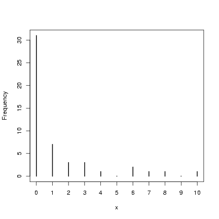
> x = rnbinom(50, mu = mu.true, size = k.true)

Take a quick look at what we got:

> plot(table(factor(x, levels = 0:max(x))), ylab = "Frequency", 
+     xlab = "x")

(reminder: I won't always draw the pictures, but it's good to make a habitat of examining your variables (with summary() etc. and graphically) as you go along to make sure you know what's going on!)

Negative log-likelihood function for a simple draw from a negative binomial distribution: the first parameter, p, will be the vector of parameters, and the second parameter, dat, will be the data vector (in case we want to try this again later with a different set of data; by default we'll set it to the x vector we just drew randomly).

> NLLfun1 = function(p, dat = x) {
+     mu = p[1]
+     k = p[2]
+     -sum(dnbinom(x, mu = mu, size = k, log = TRUE))
+ }

Calculate the negative log-likelihood for the true values. I have to combine these values into a vector with c() to pass them to the negative log-likelihood function. Naming the elements in the vector is optional but will help keep things clear as we go along:

> nll.true = NLLfun1(c(mu = mu.true, k = k.true))
> nll.true

[1] 72.64764

The NLL for other parameter values that I know are way off (

μ = 10

k = 10

> NLLfun1(c(mu = 10, k = 10))

[1] 291.4351

Much higher negative log-likelihood, as it should be.

Find the method-of-moments estimates for

μ

and

k

> m = mean(x)
> v = var(x)
> mu.mom = m
> k.mom = m/(v/m - 1)

Negative log-likelihood estimate for method of moments parameters:

> nll.mom = NLLfun1(c(mu = mu.mom, k = k.mom))
> nll.mom

[1] 72.08996

Despite the known bias, this estimate is better (lower negative log-likelihood) than the "true" parameter values. The Likelihood Ratio Test would say, however, that the difference in likelihoods would have to be greater than

χ_{2}^{2} (0.95) / 2

(two degrees of freedom because we are allowing both

μ

and

k

to change):

> ldiff = nll.true - nll.mom
> ldiff

[1] 0.5576733

> qchisq(0.95, df = 2)/2

[1] 2.995732

So - better, but not significantly better at

p = 0.05

. (pchisq(2*ldiff,df=2,lower.tail=FALSE) would tell us the exact

p

-value if we wanted to know.)

But what is the MLE? Use optim with the default options (Nelder-Mead simplex method) and the method-of-moments estimates as the starting estimates (par):

> O1 = optim(fn = NLLfun1, par = c(mu = mu.mom, k = k.mom), hessian = TRUE)
> O1

$par
       mu         k 
1.2602356 0.2884793 

$value
[1] 71.79646

$counts
function gradient 
      45       NA 

$convergence
[1] 0

$message
NULL

$hessian
            mu            k
mu 7.387808331  0.004901569
k  0.004901569 97.372581408

The optimization result is a list with elements:

the best-fit parameters (O1$par, with parameter names because we named the elements of the starting vector-see how useful this is?);
the minimum negative log-likelihood (O1$value);
information on the number of function evaluations (O1$counts; the gradient part is NA because we didn't specify a function to calculate the derivatives (and the Nelder-Mead algorithm wouldn't have used them anyway);
information on whether the algorithm thinks it found a good answer (O1$convergence, which is zero if R thinks everything worked and uses various numeric codes (see ?optim for details) if something goes wrong;
O1$message which may give further information about the when the fit converged or how it failed to converge;
because we set hessian=TRUE, we also get O1$hessian, which gives the (finite difference approximation of) the second derivatives evaluated at the MLE

The minimum negative log-likelihood (71.8) is better than either the negative log-likelihood corresponding to the method-of-moments parameters (72.09) or the true parameters (72.65), but all of these are within the LRT cutoff.

Now let's find the likelihood surface, the profiles, and the confidence intervals.

The likelihood surface is straightforward: set up vectors of

μ

and

k

values and run for loops, set up a matrix to hold the results, and run for loops to calculate and store the values. Let's try

μ

from 0.4 to 3 in steps of 0.05 and

k

from 0.01 to 0.7 in steps of 0.01. (I initially had the

μ

vector from 0.1 to 2.0 but revised it after seeing the contour plot below.)

> muvec = seq(0.4, 3, by = 0.05)
> kvec = seq(0.01, 0.7, by = 0.01)

The matrix for the results will have rows corresponding to

μ

and columns corresponding to

k

> resmat = matrix(nrow = length(muvec), ncol = length(kvec))

Run the for loops:

> for (i in 1:length(muvec)) {
+     for (j in 1:length(kvec)) {
+         resmat[i, j] = NLLfun1(c(muvec[i], kvec[j]))
+     }
+ }

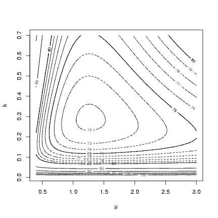
Drawing a contour: the initial default choice of contours doesn't give us fine enough resolution (it picks contours spaced 5 apart to cover the range of the values in the matrix), so I added levels spaced 1 log-likelihood unit apart from 70 to 80 by doing a second contour plot with add=TRUE.

> contour(muvec, kvec, resmat, xlab = expression(mu), ylab = "k")
> contour(muvec, kvec, resmat, levels = 70:80, lty = 2, add = TRUE)

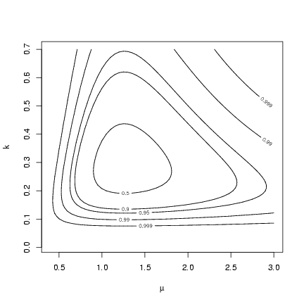
Alternately, we could set the levels of the contour plot corresponding to different

1 - α

levels for the likelihood ratio test: if the minimum negative log-likelihood is

m

, then these levels are

m + χ_{2}^{2} (α) / 2

> alevels = c(0.5, 0.9, 0.95, 0.99, 0.999)
> minval = O1$value
> nll.levels = qchisq(alevels, df = 2)/2 + minval
> contour(muvec, kvec, resmat, levels = nll.levels, labels = alevels, 
+     xlab = expression(mu), ylab = "k")

So far, so good. Finding the profiles and confidence limits is a bit harder.

To calculate the

μ

profile, define a new function that takes

μ

as a separate parameter (which optim will not try to adjust as it goes along) and optimizes with respect to

k

> NLLfun.mu = function(p, mu) {
+     k = p[1]
+     -sum(dnbinom(x, mu = mu, size = k, log = TRUE))
+ }

Set up a matrix with two columns (one for the best-fit

k

value, one for the minimum negative log-likelihood achieved):

> mu.profile = matrix(ncol = 2, nrow = length(muvec))

Run a for loop, starting the optimization from the maximum-likelihood value of

k

every time. Also include the value for

μ

(mu=muvec[i]), which R will pass on to the function that computes the negative log-likelihood.

The default Nelder-Mead method doesn't work well on 1-dimensional problems, and will give a warning. I tried method="BFGS" instead but got warnings about NaNs produced in ... , because optim tries some negative values for

k

on its way to the correct (positive) answer. I then switched to L-BFGS-B and set lower=0.002, far enough above zero that optim wouldn't run into any negative numbers when it calculated the derivatives by finite differences. Another option would have been to change the function around so that it minimized with respect to

\log (k)

instead of

k

. This function would look something like:

> NLLfun.mu2 = function(p, mu) {
+     logk = p[1]
+     k = exp(logk)
+     -sum(dnbinom(x, mu = mu, size = k, log = TRUE))
+ }

and of course we would have to translate the answers back from the log scale to compare them to the results so far. (The other option would be to use optimize, a function specially designed for 1D optimization, but this way we have to do less rearranging of the code.)

A general comment about warnings: it's OK to ignore warnings if you understand exactly where they come from and have satisfied yourself that whatever problem is causing the warnings does not affect your answer in any significant way. Ignoring warnings at any other time is a good way to overlook bugs in your code or serious problems with numerical methods that will make your answers nonsensical.

So, anyway - run that optimization for each value of

μ

in the

μ

vector. At each step, save the parameter estimate and the minimum negative log-likelihood:

> for (i in 1:length(muvec)) {
+     Oval = optim(fn = NLLfun.mu, par = O1$par["k"], method = "L-BFGS-B", 
+         lower = 0.002, mu = muvec[i])
+     mu.profile[i, ] = c(Oval$par, Oval$value)
+ }
> colnames(mu.profile) = c("k", "NLL")

Do the same process for

k

> NLLfun.k = function(p, k) {
+     mu = p[1]
+     -sum(dnbinom(x, mu = mu, size = k, log = TRUE))
+ }
> k.profile = matrix(ncol = 2, nrow = length(kvec))
> for (i in 1:length(kvec)) {
+     Oval = optim(fn = NLLfun.k, par = O1$par["mu"], method = "L-BFGS-B", 
+         lower = 0.002, k = kvec[i])
+     k.profile[i, ] = c(Oval$par, Oval$value)
+ }
> colnames(k.profile) = c("mu", "NLL")

Redraw the contour plot with profiles added:

> contour(muvec, kvec, resmat, xlab = expression(mu), ylab = "k")
> contour(muvec, kvec, resmat, levels = 70:80, lty = 2, add = TRUE)
> lines(muvec, mu.profile[, "k"], lwd = 2)
> lines(k.profile[, "mu"], kvec, lwd = 2, lty = 2)

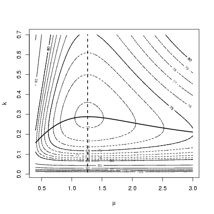The contour for

μ

is completely independent of

k

: no matter what value you choose for

k

, the best estimate of

μ

is still the same (and equal to the mean of the observed data). In contrast, values of

μ

either above or below the best value lead to estimates of

k

that are lower than the MLE.

Exercise 1: Redraw the contour plot of the likelihood surface for this data set with the contours corresponding to

α

levels, as above. Add points corresponding to the location of the MLE, the method-of-moments estimate, and the true values. State your conclusions about the differences among these 3 sets of parameters and their statistical significance.

2 Univariate profiles

Now we'd like to find the univariate confidence limits on

μ

and

k

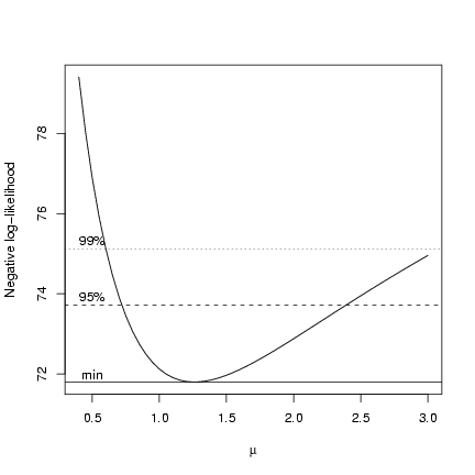
. It's easy enough to get an approximate idea of this graphically. For example, for

μ

, plotting the profile and superimposing horizontal lines for the minimum NLL and the 95% and 99% LRT cutoffs:

> plot(muvec, mu.profile[, "NLL"], type = "l", xlab = expression(mu), 
+     ylab = "Negative log-likelihood")
> cutoffs = c(0, qchisq(c(0.95, 0.99), 1)/2)
> nll.levels = O1$value + cutoffs
> abline(h = nll.levels, lty = 1:3)
> text(rep(0.5, 3), nll.levels + 0.2, c("min", "95%", "99%"))

But how do we find the

x

-intercepts (

μ

values) associated with the points where the likelihood profile crosses the cutoff lines?

Three possibilities:

If we have sampled the profile at a fairly fine scale, we can just look for the point(s) that are closest to the cutoff value:
```
> cutoff = O1$value + qchisq(0.95, 1)/2
 
```
The which.min function gives the index of the smallest element in the vector: if we find the index corresponding to the smallest value of the absolute value of the profile negative log-likelihood minus the cutoff, that should give us the μ value closest to the confidence limit. We actually need to to do this for each half of the curve separately. First the lower half, selecting values from muvec and mu.profile corresponding to values less than 1.2 (based on looking at the plot.
```
> lowerhalf = mu.profile[muvec < 1.2, "NLL"]
> lowerhalf.mu = muvec[muvec < 1.2]
> w.lower = which.min(abs(lowerhalf - cutoff))
 
```
The same thing for the upper half of the curve:
```
> upperhalf = mu.profile[muvec > 1.2, "NLL"]
> upperhalf.mu = muvec[muvec > 1.2]
> w.upper = which.min(abs(upperhalf - cutoff))
> ci.crude = c(lowerhalf.mu[w.lower], upperhalf.mu[w.upper])
 
```
Plot it:
```
> plot(muvec, mu.profile[, "NLL"], type = "l", xlab = expression(mu), 
+     ylab = "Negative log-likelihood")
> cutoffs = c(0, qchisq(c(0.95), 1)/2)
> nll.levels = O1$value + cutoffs
> abline(h = nll.levels, lty = 1:2)
> abline(v = ci.crude, lty = 3)
 
```
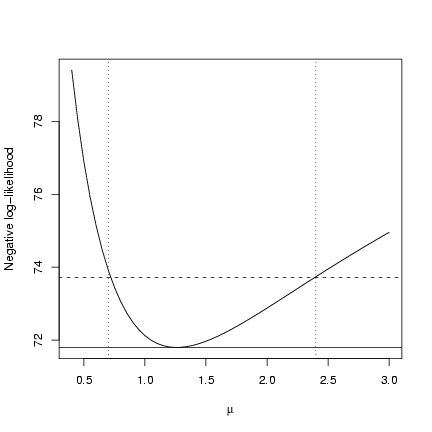You can see that it's not exactly on target, but very close. If you wanted to proceed in this way and needed a more precise answer you could "zoom in" and evaluate the profile on a finer grid around the lower and upper confidence limits.

You can set up an automatic search routine in R to try to find the confidence limits.

First, define a function that takes a particular value of

μ

, optimizes with respect to

k

, and returns the value of the negative log-likelihood minus the cutoff value, which tells us how far above or below the cutoff we are.

> cutoff = O1$value + qchisq(c(0.95), 1)/2
> relheight = function(mu) {
+     O2 = optim(fn = NLLfun.mu, par = O1$par["k"], method = "L-BFGS-B", 
+         lower = 0.002, mu = mu)
+     O2$value - cutoff
+ }

We know the lower limit is somewhere around 0.7, so going on either side should give us values that are negative/positive.

> relheight(mu = 0.6)

[1] 1.420474

> relheight(mu = 0.8)

[1] -0.6530479

Using R's uniroot function, which takes a single-parameter function and searches for a value that gives zero:

> lower = uniroot(relheight, interval = c(0.5, 1))$root
> upper = uniroot(relheight, interval = c(1.2, 5))$root
> ci.uniroot = c(lower, upper)

> plot(muvec, mu.profile[, "NLL"], type = "l", xlab = expression(mu), 
+     ylab = "Negative log-likelihood")
> cutoffs = c(0, qchisq(c(0.95), 1)/2)
> nll.levels = O1$value + cutoffs
> abline(h = nll.levels, lty = 1:2)
> abline(v = ci.crude, lty = 3)
> abline(v = ci.uniroot, lty = 4)

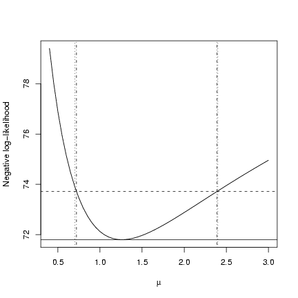Slightly more precise than the previous solution.

Using the information-based approach. Here is the information matrix:
```
> O1$hessian
 
```
```
            mu            k
mu 7.387808331  0.004901569
k  0.004901569 97.372581408

 
```
Inverting the information matrix:
```
> s1 = solve(O1$hessian)
> s1
 
```
```
              mu             k
mu  1.353581e-01 -6.813697e-06
k  -6.813697e-06  1.026983e-02

 
```
You can see that the off diagonal elements are very small ( -6× 10-6 as opposed to 0.0102 and 0.135 on the diagonal), correctly suggesting that the parameter estimates are uncorrelated.
Suppose we want to approximate the likelihood profile by the quadratic L=a+c(μ-b )2 . The parameter b governs the μ value at which the minimum occurs (so b corresponds to the MLE of μ) and parameter a governs the height of the minimum (so a is the minimum negative log-likelihood). The second derivative of the quadratic is 2c; the second derivative of the likelihood surface is ∂2 L/∂ μ2 , so c=( ∂2 L/∂ μ2 )/2.
```
> a = O1$value
> b = O1$par["mu"]
> c = O1$hessian["mu", "mu"]/2
 
```
We get the variances of the parameters ( σμ 2 , σk 2 ) by inverting the information matrix. The size of the confidence limit is ±1.96 σμ for 95% confidence limits, or more generally ± qnorm(1-alpha/2) σμ (qnorm gives the quantile of the standard normal, with mean 0 and standard deviation 1, by default).
```
> se.mu = sqrt(s1["mu", "mu"])
> ci.info = O1$par["mu"] + c(-1, 1) * qnorm(0.975) * se.mu
 
```
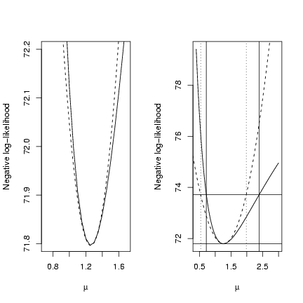
Double plot, showing a close-up of the negative log-likelihood minimum (to convince you that the quadratic approximation really is a good fit if you go close enough to the minimum - this is essentially a Taylor expansion, provided that the likelihood surface is reasonably well-behaved) and a wider view comparing the quadratic approximation and the confidence limits based on
```
> op = par(mfrow = c(1, 2))
> plot(muvec, mu.profile[, "NLL"], type = "l", xlab = expression(mu), 
+     ylab = "Negative log-likelihood", ylim = c(71.8, 72.2), xlim = c(0.7, 
+         1.7))
> curve(a + c * (x - b)^2, add = TRUE, lty = 2)
> plot(muvec, mu.profile[, "NLL"], type = "l", xlab = expression(mu), 
+     ylab = "Negative log-likelihood")
> cutoffs = c(0, qchisq(c(0.95), 1)/2) + O1$value
> curve(a + c * (x - b)^2, add = TRUE, lty = 2)
> abline(h = cutoffs)
> abline(v = ci.info, lty = 3)
> abline(v = ci.uniroot, lty = 1)
> par(op)
 
```
One way to cheat: use the fitdistr function from the MASS package instead (this only works for simple draws from distributions).
```
> library(MASS)
> f = fitdistr(x, "negative binomial")
> f
 
```
```
     size         mu    
  0.2885187   1.2597788 
 (0.1013610) (0.3676483)

 
```
fitdistr gives the parameters in the other order - size and mu rather than mu and k as I have been naming them. It gives standard errors based on the quadratic approximation, so the same as by the previous method. (I had to use str(f) to look inside f and figure out how to extract the numbers I wanted.)
```
> ci.fitdistr = f$estimate["mu"] + c(-1, 1) * f$sd["mu"] * qnorm(0.975)
 
```
The last option is to use the mle function from the stats4 package to find the confidence intervals. To do this, we have to rewrite the NLL function slightly differently: (1) specify the parameters separately, rather than packing them into a parameter vector (and then unpacking them inside the function - so this is actually slightly more convenient), and (2) you can't pass the data as additional argument: if you want to run the function for another set of data you have to replace x with your new data, or write another function (there are other kinds of black magic you can do to achieve the same goal, but they are too complicated to lay out here (P2C2E [1])).
```
> NLLfun2 = function(mu, k) {
+     -sum(dnbinom(x, mu = mu, size = k, log = TRUE))
+ }
 
```
mle has slightly different argument names from optim, but you still have to specify the function and the starting values, and you can include other options (which get passed straight to optim):
```
> library(stats4)
> m1 = mle(minuslogl = NLLfun2, start = list(mu = mu.mom, k = k.mom), 
+     method = "L-BFGS-B", lower = 0.002)
> m1
 
```
```
Call:
mle(minuslogl = NLLfun2, start = list(mu = mu.mom, k = k.mom), 
    method = "L-BFGS-B", lower = 0.002)

Coefficients:
       mu         k 
1.2600009 0.2885231 

 
```
summary(m1) gives the estimates and the standard errors based on the quadratic approximation:
```
> summary(m1)
 
```
```
Maximum likelihood estimation

Call:
mle(minuslogl = NLLfun2, start = list(mu = mu.mom, k = k.mom), 
    method = "L-BFGS-B", lower = 0.002)

Coefficients:
    Estimate Std. Error
mu 1.2600009  0.3677636
k  0.2885231  0.1013633

-2 log L: 143.5929 

 
```
confint(m1) gives the profile confidence limits, for all parameters (the second line below takes just the row corresponding to mu).
```
> ci.mle.all = confint(m1)
 
```
```
Profiling...

 
```
```
> ci.mle.all
 
```
```
       2.5 %   97.5 %
mu 0.7204352 2.390998
k  0.1437419 0.579509

 
```
```
> ci.mle = ci.mle.all["mu", ]
 
```
The confint code is based on first calculating the profile (as we did above, but at a smaller number of points), then using spline-based interpolation to find the intersections with the cutoff height.

Comparing all of these methods:

> citab = rbind(ci.crude, ci.uniroot, ci.mle, ci.info, ci.fitdistr)
> citab

                2.5 %   97.5 %
ci.crude    0.7000000 2.400000
ci.uniroot  0.7200252 2.390702
ci.mle      0.7204352 2.390998
ci.info     0.5391442 1.981327
ci.fitdistr 0.5392013 1.980356

3 Reef fish: settler distribution

Let's simulate the reef fish data again:

> a = 0.696
> b = 9.79
> recrprob = function(x, a = 0.696, b = 9.79) a/(1 + (a/b) * x)
> scoefs = c(mu = 25.32, k = 0.932, zprob = 0.123)
> settlers = rzinbinom(603, mu = scoefs["mu"], size = scoefs["k"], 
+     zprob = scoefs["zprob"])
> recr = rbinom(603, prob = recrprob(settlers), size = settlers)

Set up likelihood functions - let's say we know the numbers of settlers and are trying to estimate the recruitment probability function. I'll use mle.

First, a Shepherd function:

> NLLfun3 = function(a, b, d) {
+     recrprob = a/(1 + (a/b) * settlers^d)
+     -sum(dbinom(recr, prob = recrprob, size = settlers, log = TRUE), 
+         na.rm = TRUE)
+ }

> NLLfun4 = function(a, b) {
+     recrprob = a/(1 + (a/b) * settlers)
+     -sum(dbinom(recr, prob = recrprob, size = settlers, log = TRUE), 
+         na.rm = TRUE)
+ }

> NLLfun5 = function(a) {
+     recrprob = a
+     -sum(dbinom(recr, prob = recrprob, size = settlers, log = TRUE), 
+         na.rm = TRUE)
+ }

I ran into a problem with this log-likelihood function: when settlers=0, the recruitment probability is

a

, which may be greater than 0. This doesn't matter in reality because when there are zero settlers there aren't any recruits. From a statistical point of view, the probability of zero recruits is 1 when there are zero settlers, but dbinom(x,prob=a,size=0) still comes out with NaN. However, since I know what the problem is and I know that the log-likelihood in this case is

\log (1) = 0

and so contributes nothing to the log-likelihood, I am safe using the na.rm=TRUE option for sum. However, this does still gives me warnings about NaNs produced in: dbinom ... . A better solution might be to drop the zero-settler cases from the data entirely:

> recr = recr[settlers > 0]
> settlers = settlers[settlers > 0]

> plot(settlers, recr)
> abline(h = 10)
> abline(a = 0, b = 0.5)

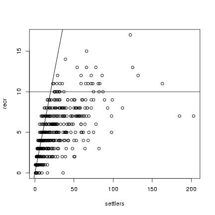Looking at a plot of the data, I can eyeball the asymptote (

b

) at about 10 recruits, the initial slope (

a

) at about 0.5, and I'll start with

d = 1

Had to mess around a bit - fitted the simpler (Beverton-Holt) model first, and found I had to use L-BFGS-B to get mle not to choke while computing the information matrix.

> m4 = mle(minuslogl = NLLfun4, start = list(a = 0.5, b = 10), 
+     method = "L-BFGS-B", lower = 0.003)
> s3 = list(a = 0.684, b = 10.161, d = 1)
> m3 = mle(minuslogl = NLLfun3, start = s3, method = "L-BFGS-B", 
+     lower = 0.003)
> m5 = mle(minuslogl = NLLfun5, start = list(a = 0.5), method = "L-BFGS-B", 
+     lower = 0.003)

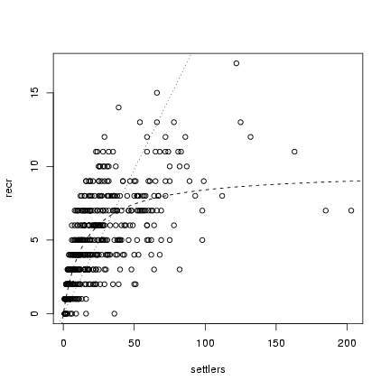
Plot all fits against the data:

> plot(settlers, recr)
> a = coef(m5)["a"]
> curve(a * x, add = TRUE, lty = 3)
> a = coef(m4)["a"]
> b = coef(m4)["b"]
> curve(a * x/(1 + (a/b) * x), add = TRUE, lty = 2)
> a = coef(m5)["a"]
> b = coef(m5)["b"]
> d = coef(m5)["d"]
> curve(a * x/(1 + (a/b) * x^d), add = TRUE, lty = 3)

Compare the negative log-likelihoods:

> nll = c(shep = -logLik(m3), BH = -logLik(m4), densind = -logLik(m5))
> nll

    shep       BH  densind 
1020.427 1020.843 1444.717

As required, the Shepherd has a better likelihood than the Beverton-Holt, but only by a tiny amount - certainly not greater than the LRT cutoff. On the other hand, there is extremely strong support for density-dependence, from the 424 log-likelihood-unit differences between the density-independent and Beverton-Holt model likelihoods. It's silly, but you can calculate the logarithm of the

p

-value as:

> logp = pchisq(2 * nll[3] - nll[2], 1, lower.tail = FALSE, log.p = TRUE)
> logp

 densind 
-938.288

That's equivalent to

p \approx 10^{- 407.36822402525}

(there's a much higher probability that the CIA broke into your computer and tampered with your data).

We would get the same answer by calculating AIC values:

> npar = c(5, 4, 3)
> aic = nll + 2 * npar
> aic

    shep       BH  densind 
1030.427 1028.843 1450.717

Or BIC values:

> ndata = length(recr)
> bic = nll + log(ndata) * npar
> bic

    shep       BH  densind 
1051.609 1045.788 1463.426

(except that BIC says more strongly that the Shepherd is not worth considering in this case).

The confidence intervals tell the same story:

> confint(m3)

Profiling...
      2.5 %     97.5 %
a 0.5804655  0.8629449
b 4.5161010 13.2424549
d 0.8183632  1.0738295

the 95% confidence intervals of

d

include 1 (just).

> confint(m4)

Profiling...
      2.5 %     97.5 %
a 0.5833164  0.7180549
b 8.9412876 10.4844295

We get tighter bounds on

a

with the Beverton-Holt model (since we are not wasting data trying to estimate

d

), and we get reasonable bounds on

b

. (When I used BFGS instead of L-BFGS-B, even though I got reasonable answers for the MLE, I ran into trouble when I tried to get profile confidence limits.) In particular, the upper confidence interval of

b

< \infty

(which it would not be if the density-independent model were a better fit).

Exercise 2: redo the fitting exercise, but instead of using L-BFGS-B, fit log

a

, log

b

, and log

d

to avoid having to use constrained optimization. Back-transform your answers for the point estimates and the confidence limits by exponentiating; make sure they check closely with the answers above.

Exercise 3: fit zero-inflated negative binomial, negative binomial, and Poisson distributions to the settler data. State how the three models are nested; perform model selection by AIC and LRT, and compare the confidence intervals of the parameters. What happens if you simulate half as much "data"?

References

[1]: Salman Rushdie. Haroun and the Sea of Stories. Faber & Faber, 1999.

File translated from T_EX by T_TM, version 3.70.
On 20 Oct 2005, 02:12.