 > ellipse()
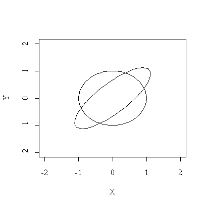
 > ellipse(1.5, 0.5, pi/4)
The function ellipse() adds an ellipse to the current plot and has the following arguments:
hlaxa    half-length of the major axis (parallel to the X-axis
         when theta = 0)

hlaxb    half-length of the minor axis

theta    angle of rotation, measured counter-clockwise from the
         positive X-axis

xc       the X-coordinate of the centre

yc       the Y-coordinate of the centre

npoints  the number of line segments used to approximate the ellipse
As the angle a is incremented evenly in npoints steps from 0 to 2*pi, the (x, y) coordinates are computed for points around the circumference of an ellipse centred at the origin and parallel to the axes. If the angle of rotation theta is non-zero, each (x, y) pair is converted to polar coordinates (rad, alpha) using the function angle(), rotated by angle theta around the origin, then reconverted to rectangular coordinates (x, y). If the ellipse is not centred on the origin, the (x, y) coordinates are shifted by (xc, yc) when they are accumulated in vectors (xp, yp).
> ellipse <-
function(hlaxa = 1, hlaxb = 1, theta = 0, xc = 0, yc = 0, npoints = 100)
{
        xp <- NULL
        yp <- NULL
        for(i in 0:npoints) {
                a <- (2 * pi * i)/npoints
                x <- hlaxa * cos(a)
                y <- hlaxb * sin(a)
                if(theta != 0) {
                        alpha <- angle(x, y)
                        rad <- sqrt(x^2 + y^2)
                        x <- rad * cos(alpha + theta)
                        y <- rad * sin(alpha + theta)
                }
                xp <- c(xp, x + xc)
                yp <- c(yp, y + yc)
        }
        lines(xp, yp, type = "l")
        invisible()
}

> angle <-
function(x, y)
{
        if(x > 0) {
                atan(y/x)
        }
        else {
                if(x < 0 & y != 0) {
                        atan(y/x) + sign(y) * pi
                }
                else {
                        if(x < 0 & y == 0) {
                                pi
                        }
                        else {
                                if(y != 0) {
                                        (sign(y) * pi)/2
                                }
                                else {
                                        NA
                                }
                        }
                }
        }
}
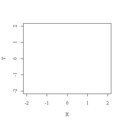
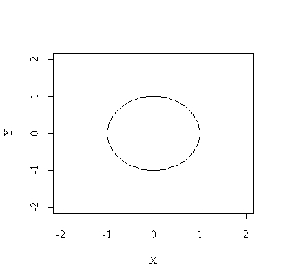
Here we see how ellipse() is used. Note that ellipse() adds the ellipse to an existing plot, so in this example we begin by creating a plot with the required dimensions but no points or lines (type = "n"), then add the default ellipse, a unit circle, which looks elliptical because the plot area is not isometric, and finally add an ellipse with axis half-lengths 1.5 and 0.5 rotated by pi/4 but centred on the origin.
> plot(c(-2,2), c(-2,2), xlab="X", ylab="Y", type="n")
Often we are given an equation with a quadratic form (x - m)'A(x - m) = c2 and we want to draw the ellipse it defines. The function ellipsem() does the required eigenanalysis on the matrix of the quadratic form and calls ellipse() to draw the ellipse.
> ellipsem <-
function (mu, amat, c2, npoints = 100)
{
    if (dim(amat) == c(2, 2)) {
        eamat <- eigen(amat)
        hlen <- sqrt(c2/eamat$val)
        theta <- angle(eamat$vec[1, 1], eamat$vec[2, 1])
        ellipse(hlen[1], hlen[2], theta, mu[1], mu[2], npoints = npoints)
    }
    invisible()
}
Here is an example; we have bone density measured in the non-dominant radius and humerus of 25 subjects. This code draws a scatterplot, marks the mean with a "+", and draws the 95% confidence ellipse for the population mean.
> plot(radius, humerus)
> points(mean(radius), mean(humerus), pch="+")
> n <- length(radius)
> p <- 2
> ellipsem(c(mean(radius), mean(humerus)), solve(var(cbind(radius,humerus))), ((n-1)*p/(n-p))*qf(0.95,p,n-p)/n)