Mean (variance known).
Mean (variance unknown).
Mean difference (variance unknown).
Difference in means (variances known).

Difference in means (variances unknown, homoscedastic).

Variance (mean unknown).
Ratio of variances (means unknown).
The marking scheme is indicated in red. Full Marks = 50.
(a) Define the following terms: homoscedasticity, parameter, statistic, sampling distribution, pivotal quantity. [5 marks]
Homoscedasticity means that the variance of a random variable is the same in each subpopulation or at any given level of the covariates.
A parameter is a scalar or vector that indexes a family of probability distributions.
A statistic is any function of the observations in a sample. It may not include any unknown parameters.
The distribution of a statistic is called a sampling distribution. It describes how the statistic will vary from one sample to another.
A pivotal quantity is a function of a statistic and the parameter of interest that follows a standard distribution. The distribution may not include any unknown parameters.
(b) Give one example of a pivotal quantity, and write out the confidence interval formula derived from it. [5 marks]
Any one of the following examples will do.
|
|
|
|
|
Mean (variance known). |
|
|
|
Mean (variance unknown). |
|
|
|
Mean difference (variance unknown). |
|
|
|
Difference in means (variances known). |

|
|
|
Difference in means (variances unknown, homoscedastic). |

|
|
|
Variance (mean unknown). |
|
|
|
Ratio of variances (means unknown). |
|
|
(a) Student's t distribution was discovered by an applied chemist named William Sealy Gosset. Why wasn't it called Gosset's t? [2 marks]
Gosset was employed by the Guinness brewery. Guinness did not want him publishing in his own name, for fear of revealing trade secrets, so he published his work on the t-distribution under the pseudonym of "Student".
(b) What applied problem motivated Gosset to study the Poisson distribution? [2 marks]
He was using a hemocytometer to count yeast cells at the brewery and he was interested in the variation between observations.
(c) What two professions claim Florence Nightingale as a pioneer? [1 mark]
Nursing and Medical Statistics.
Analyse the following two data sets with appropriate graphics and 95% confidence intervals. State your assumptions and your conclusions. Where possible, assess the validity of your assumptions. [30 marks]
(a) Ten tires of Brand A and 8 tires of Brand B were road-tested to determine tread life in units of 100 km.
The analysis is difference of means for two independent samples, assuming independence, normality, homoscedasticity.
Graphical analysis: comparative dot plot or comparative box plot.
- Independence: can't test; if the tires aren't in any serial order, testing for autocorrelation won't be possible.
- Normality: could draw histograms or stem-leaf plots but the comparative dot plot or comparative box plot (shown) is enough to indicate that the two distributions are reasonably symmetric and free of outliers.
- Homoscedasticity: do a confidence interval for the ratio of variances.
95% confidence interval for the difference in means:
> xbara <- mean(tires$life[tires$brand=="A"])
> xbarb <- mean(tires$life[tires$brand=="B"])
> s2a <- var(tires$life[tires$brand=="A"])
> s2b <- var(tires$life[tires$brand=="B"])
> xbara
[1] 61.65
> xbarb
[1] 60.025
> s2a
[1] 6.849444
> s2b
[1] 16.57643
> sp <- sqrt((9*s2a+7*s2b)/16)
> xbara-xbarb + c(-1,1)*qt(.975,16)*sp*sqrt((1/10)+(1/8))
[1] -1.725943  4.975943
The confidence interval includes 0 so we conclude that there is no evidence of a difference in mean life between brands, at the 95% level of confidence.
95% confidence interval for the ratio of variances:
> c((s2a/s2b)/qf(.975,9,7), (s2a/s2b)/qf(.025,9,7))
[1] 0.08566976 1.73423591
The confidence interval includes 1 so there is no evidence of heteroscedasticity, at the 95% level of confidence.
(b) An industrial safety program was instituted in 10 similar factories. The number of employee hours lost due to accidents per week (averaged over one month) was recorded at each plant before and after the program. The factories are listed in no particular order.
The analysis is a 95% confidence interval for the mean difference, from paired data. You could also give a confidence interval for the mean ratio or the mean difference in logs.
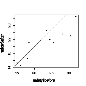
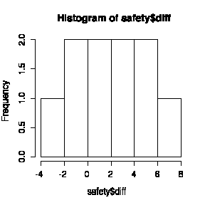
Graphical analysis: a scatter plot of "After" versus "Before", and a dot plot or box plot or histogram of the differences. Since the factories are listed in no particular order, a series plot or lag-1 plot would NOT be appropriate.
> safety
   before after diff     ratio
1    30.5  23.0  7.5 1.3260870
2    18.5  21.0 -2.5 0.8809524
3    24.5  22.0  2.5 1.1136364
4    32.0  28.5  3.5 1.1228070
5    16.0  14.5  1.5 1.1034483
6    15.0  15.5 -0.5 0.9677419
7    23.5  24.5 -1.0 0.9591837
8    25.5  21.0  4.5 1.2142857
9    28.0  23.5  4.5 1.1914894
10   18.0  16.5  1.5 1.0909091

> plot(safety$before,safety$after,pch=19)
> abline(0,1)
> hist(safety$diff)


- Independence: can't test.
- Normality: the histogram (or box plot or dot plot) is symmetric and free of outliers, so the assumption of normality is reasonable.
- Constant mean difference: the points at the top right of the scatter plot tend to lie further below the diagonal than the points at the bottom left, suggesting that the magnitude of the difference increases with the "Before" level, so an analysis of ratios or differences in logs, rather than arithmetic differences, is justified but not required.
95% Confidence Interval for the mean difference:
> mean(safety$diff) + c(-1,1)*qt(.975,9)*sqrt(var(safety$diff)/10)
[1] 0.003598135 4.296401865
The 95% confidence interval for the difference does not include 0, so there is evidence at the 95% level of confidence that the program reduces the mean hours lost.
95% Confidence Interval for the ratio:
> mean(safety$ratio) + c(-1,1)*qt(.975,9)*sqrt(var(safety$ratio)/10)
[1] 1.002102 1.192006
The 95% confidence interval for the ratio does not include 1, so the conclusion is the same.
95% Confidence Interval for the log ratio:
> mean(log(safety$ratio)) + c(-1,1)*qt(.975,9)*sqrt(var(log(safety$ratio))/10)
[1] -0.001797388  0.173655843
The 95% confidence interval for the log ratio (or difference in logs) does include 0, so that analysis tdoes not give evidence that the program reduces the mean hours lost.
Any ONE of these three confidence intervals and its conclusion will be enough.
Suppose that you are going to repeat the study described in 3(b) but this time you want the confidence interval for the mean difference to be ± 1 hour lost. How many factories will you need? [5 marks]
Taking s2d = 9.00 and t0.025, n-1 = 2 as the best available values, solve for n in t0.025, n-1 * sd / sqrt(n) = 1 to get
n = (2*3)2 = 36.