Updated 1998-04-08
A consumer product-testing organization compared the annual power consumption for five different brands of dehumidifier. As far as possible, comparable models were chosen from each manufacturer. Eight units of each model were purchased from randomly-chosen retail outlets. Because power consumption depends on the prevailing humidity level, each model was tried at four different levels, ranging from moderate to high humidity, two units being assigned at random to each humidity level. The table below shows annual power consumption in kwh for each of the 40 units tested.
|
|
|
Humidity |
|
|
|
|
|
|
1 |
2 |
3 |
4 |
|
Brand |
1 |
661, 690 |
779, 782 |
848, 833 |
841, 854 |
|
|
2 |
760, 732 |
791, 788 |
878, 894 |
983, 953 |
|
|
3 |
742, 751 |
806, 808 |
906, 902 |
984, 953 |
|
|
4 |
775, 827 |
879, 887 |
931, 950 |
1029, 970 |
|
|
5 |
842, 795 |
956, 916 |
983, 989 |
1012, 1039 |
The data are entered in the MINITAB worksheet in three columns as shown below, one column to each variable, one row to each unit. The ANOVA command is all that is needed to produce an ANOVA table with main effects and interaction.
MTB > Print 'kwh' 'brand' 'humidity'.

 ROW    kwh  brand  humidity

   1    661      1         1
   2    690      1         1
   3    760      2         1
   4    732      2         1
   5    742      3         1
   6    751      3         1
   7    775      4         1
   8    827      4         1
   9    842      5         1
  10    795      5         1
  11    779      1         2
  12    782      1         2
  13    791      2         2
  14    788      2         2
  15    806      3         2
  16    808      3         2
  17    879      4         2
  18    887      4         2
  19    956      5         2
  20    916      5         2
  21    848      1         3
  22    833      1         3
  23    878      2         3
  24    894      2         3
  25    906      3         3
  26    902      3         3
  27    931      4         3
  28    950      4         3
  29    983      5         3
  30    989      5         3
  31    841      1         4
  32    854      1         4
  33    983      2         4
  34    953      2         4
  35    984      3         4
  36    953      3         4
  37   1029      4         4
  38    970      4         4
  39   1012      5         4
  40   1039      5         4

MTB > ANOVA kwh = brand + humidity + brand*humidity

Factor     Type Levels Values
brand     fixed      5     1     2     3     4     5
humidity  fixed      4     1     2     3     4

Analysis of Variance for kwh

Source            DF         SS         MS       F      P
brand              4     113012      28253   73.20  0.000
humidity           3     237206      79069  204.85  0.000
brand*humidity    12      10182        849    2.20  0.058
Error             20       7720        386
Total             39     368120

MTB > noou
First, enter all 40 kwh values in your calculator and compute sum = 34699, sum of squares = 30468635. This gives you:
SST = 30468635/1 - 34699^2/40 = 368119.97
Note that there are 40 numbers in the sum, and its square is divided by 40. There is a pattern here that will see you safely through the calculations!
Note that you could also use your calculator to compute SST = (n-1)*s2
Next, go back to the table and compute the totals for each cell, row, and column. To check your work, verify that the sum of row totals and the sum of column totals each equals the sum of all observations, 34699, computed above.
|
|
|
Humidity |
|
|
|
|
|
|
|
1 |
2 |
3 |
4 |
Total |
|
Brand |
1 |
1351 |
1561 |
1681 |
1695 |
6288 |
|
|
2 |
1492 |
1579 |
1772 |
1936 |
6779 |
|
|
3 |
1493 |
1614 |
1808 |
1937 |
6852 |
|
|
4 |
1602 |
1766 |
1881 |
1999 |
7248 |
|
|
5 |
1637 |
1872 |
1972 |
2051 |
7532 |
|
|
Total |
7575 |
8392 |
9114 |
9618 |
34699 |
Use your calculator to get the sum and sum of squares of the 20 cell totals. The sum should, of course, be 34699; the sum of squares is 60921831. Each cell total is the sum of 2 numbers, so the Error sum of squares is computed as the total sum of squares divided by 1, minus the cell sum of squares divided by 2.
SSE = 30468635/1 - 60921831/2 = 7719.5
The sum of squares of row totals is 241708217. Each row total is the sum of 8 numbers, the grand total is the sum of 40 numbers, so the Row sum of squares is
SSrow = 241708217/8 - 34699^2/40 = 113012.1
The sum of squares of column totals is 303377209. Each column total is the sum of 10 numbers, the grand total is the sum of 40 numbers, so the Column sum of squares is
SScol = 303377209/10 - 34699^2/40 = 237205.87
Finally, obtain the interaction sum of squares by subtraction and complete the ANOVA table.
SSrow*col = SST - SSrow - SScol - SSE = 10182.5

 SV                 SS    DF      MS         F      P
__________________________________________________________
Brand          113012.1    4  28253.025    73.20   0.000
Humidity       237205.87   3  79068.623   204.85   0.000
Brand*Humidity  10182.5   12    848.542     2.20   0.058
Error            7719.5   20    385.975

Total          368119.97  39
The interaction is not significant at the 5% level (P = 0.058), so we can proceed to test the main effects, both of which are highly significant. Hence we conclude that the annual power consumption of dehumidifiers varies with brand and with the level of humidity, but the response to humidity is the same for each brand tested.
We were able to test the interaction in this experiment because there was replication: each brand and humidity combination had been tried twice. Had they known in advance that there was no interaction, they could have done an experiment half the size, trying each brand and humidity combination just once. This would give 0 df for Error but the 12 df for Interaction could be used as the Error term.
If we ignore Humidity and analyze the data in a one-factor ANOVA, we get the following result:; the sums of squares for Humidity and for the Interaction simply get added into the Error sum of squares.
 SV                 SS    DF      MS         F      P
__________________________________________________________
Brand          113012.1    4  28253.025    3.876   0.010
Error          255107.87  35   7288.796

Total          368119.97  39
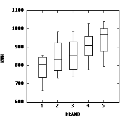
The brands are still significantly different by this analysis, but the differences have been obscured by the different humidities. The one-factor analysis can be represented graphically by the following grouped box plot.

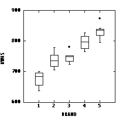
The two-factor ANOVA adjusts for differences in humidity. In the following grouped box plot, each kwh value has been adjusted by subtracting the difference between the mean for that humidity level and the mean at the lowest humidity level. This effectively standardizes all the readings to the lowest humidity level and allows the differences between brands to be seen much more clearly. This shows how much was gained by doing a two-factor analysis rather than one-factor. The graph can also be used to justify the assumptions of normality (most boxes reasonably symmetric) and homoscedasticity (dispersion in kwh is more or less the same magnitude for each brand).

Another way to graph the data and interpret the ANOVA results is to plot the mean power consumption for each brand against humidity, and the mean power consumption at each level of humidity against brand. Click here to see these results.